Example_Walkthrough
Example_Walkthrough.RmdIntroduction
In this walkthrough, we will go through the various use cases of TangledFeatures and how it outperforms traditional feature selection methods. We will also compare the raw accuracy of the package to other methods including standard black box approaches.
TangledFeatures relies on the dataset input to be correct. If there are categorical features please ensure that it is input as a factor. If done correctly, the package will identify the correct correlation based relationships between the variables.
In this example, we will be using the Boston housing prices data set. There has been some cleaning beforehand so that all the variables are in the correct orientation.
Getting Started
TangledFeatures primarily relies on ggplot2 for visualization, data.table for data manipulation, correlation for various correlation methods and ranger for its Random Forest implementation. There are a few other packages used to run certain features.
options(warn=-1)

suppressMessages(suppressWarnings(library(ranger)))
suppressMessages(suppressWarnings(library(igraph)))
suppressMessages(suppressWarnings(library(correlation)))
suppressMessages(suppressWarnings(library(data.table)))
suppressMessages(suppressWarnings(library(fastDummies)))
suppressMessages(suppressWarnings(library(ggplot2)))

suppressMessages(suppressWarnings(library(randomForest)))
suppressMessages(suppressWarnings(library(glmnet)))
suppressMessages(suppressWarnings(library(caret)))
suppressMessages(suppressWarnings(library(broom)))
suppressMessages(suppressWarnings(library(broom.mixed)))
suppressMessages(suppressWarnings(library(jtools)))
Loading the Data
To read the data we can use the simple:
data <- TangledFeatures::Housing_Prices_dataset
data <- data[,-1]
Let’s call the package’s data cleaning function. It sets dummy columns, cleans NAs and a host of other functions. You can check the ‘Data Cleaning’ tab for further information. We also need to define the dependent variable.
Data <- TangledFeatures::DataCleaning(Data = data, Y_var = 'SalePrice')Let’s see the new columns
colnames(Data$Cleaned_Data)
#>   [1] "ms_sub_class"            "lot_frontage"
#>   [3] "lot_area"                "overall_qual"
#>   [5] "overall_cond"            "year_built"
#>   [7] "year_remod_add"          "mas_vnr_area"
#>   [9] "bsmt_fin_sf1"            "bsmt_fin_sf2"
#>  [11] "bsmt_unf_sf"             "total_bsmt_sf"
#>  [13] "x1st_flr_sf"             "x2nd_flr_sf"
#>  [15] "low_qual_fin_sf"         "gr_liv_area"
#>  [17] "bsmt_full_bath"          "bsmt_half_bath"
#>  [19] "full_bath"               "half_bath"
#>  [21] "bedroom_abv_gr"          "kitchen_abv_gr"
#>  [23] "tot_rms_abv_grd"         "fireplaces"
#>  [25] "garage_yr_blt"           "garage_cars"
#>  [27] "garage_area"             "wood_deck_sf"
#>  [29] "open_porch_sf"           "enclosed_porch"
#>  [31] "x3ssn_porch"             "screen_porch"
#>  [33] "pool_area"               "misc_val"
#>  [35] "mo_sold"                 "yr_sold"
#>  [37] "sale_price"              "ms_zoning_c_all"
#>  [39] "ms_zoning_fv"            "ms_zoning_rh"
#>  [41] "ms_zoning_rl"            "ms_zoning_rm"
#>  [43] "street_grvl"             "street_pave"
#>  [45] "alley_0"                 "alley_grvl"
#>  [47] "alley_pave"              "lot_shape_ir1"
#>  [49] "lot_shape_ir2"           "lot_shape_ir3"
#>  [51] "lot_shape_reg"           "land_contour_bnk"
#>  [53] "land_contour_hls"        "land_contour_low"
#>  [55] "land_contour_lvl"        "utilities_all_pub"
#>  [57] "utilities_no_se_wa"      "lot_config_corner"
#>  [59] "lot_config_cul_d_sac"    "lot_config_fr2"
#>  [61] "lot_config_fr3"          "lot_config_inside"
#>  [63] "land_slope_gtl"          "land_slope_mod"
#>  [65] "land_slope_sev"          "neighborhood_blmngtn"
#>  [67] "neighborhood_blueste"    "neighborhood_br_dale"
#>  [69] "neighborhood_brk_side"   "neighborhood_clear_cr"
#>  [71] "neighborhood_collg_cr"   "neighborhood_crawfor"
#>  [73] "neighborhood_edwards"    "neighborhood_gilbert"
#>  [75] "neighborhood_idotrr"     "neighborhood_meadow_v"
#>  [77] "neighborhood_mitchel"    "neighborhood_n_ames"
#>  [79] "neighborhood_no_ridge"   "neighborhood_n_pk_vill"
#>  [81] "neighborhood_nridg_ht"   "neighborhood_nw_ames"
#>  [83] "neighborhood_old_town"   "neighborhood_sawyer"
#>  [85] "neighborhood_sawyer_w"   "neighborhood_somerst"
#>  [87] "neighborhood_stone_br"   "neighborhood_swisu"
#>  [89] "neighborhood_timber"     "neighborhood_veenker"
#>  [91] "condition1_artery"       "condition1_feedr"
#>  [93] "condition1_norm"         "condition1_pos_a"
#>  [95] "condition1_pos_n"        "condition1_rr_ae"
#>  [97] "condition1_rr_an"        "condition1_rr_ne"
#>  [99] "condition1_rr_nn"        "condition2_artery"
#> [101] "condition2_feedr"        "condition2_norm"
#> [103] "condition2_pos_a"        "condition2_pos_n"
#> [105] "condition2_rr_ae"        "condition2_rr_an"
#> [107] "condition2_rr_nn"        "bldg_type_1fam"
#> [109] "bldg_type_2fm_con"       "bldg_type_duplex"
#> [111] "bldg_type_twnhs"         "bldg_type_twnhs_e"
#> [113] "house_style_1_5fin"      "house_style_1_5unf"
#> [115] "house_style_1story"      "house_style_2_5fin"
#> [117] "house_style_2_5unf"      "house_style_2story"
#> [119] "house_style_s_foyer"     "house_style_s_lvl"
#> [121] "roof_style_flat"         "roof_style_gable"
#> [123] "roof_style_gambrel"      "roof_style_hip"
#> [125] "roof_style_mansard"      "roof_style_shed"
#> [127] "roof_matl_cly_tile"      "roof_matl_comp_shg"
#> [129] "roof_matl_membran"       "roof_matl_metal"
#> [131] "roof_matl_roll"          "roof_matl_tar_grv"
#> [133] "roof_matl_wd_shake"      "roof_matl_wd_shngl"
#> [135] "exterior1st_asb_shng"    "exterior1st_asph_shn"
#> [137] "exterior1st_brk_comm"    "exterior1st_brk_face"
#> [139] "exterior1st_c_block"     "exterior1st_cemnt_bd"
#> [141] "exterior1st_hd_board"    "exterior1st_im_stucc"
#> [143] "exterior1st_metal_sd"    "exterior1st_plywood"
#> [145] "exterior1st_stone"       "exterior1st_stucco"
#> [147] "exterior1st_vinyl_sd"    "exterior1st_wd_sdng"
#> [149] "exterior1st_wd_shing"    "exterior2nd_asb_shng"
#> [151] "exterior2nd_asph_shn"    "exterior2nd_brk_cmn"
#> [153] "exterior2nd_brk_face"    "exterior2nd_c_block"
#> [155] "exterior2nd_cment_bd"    "exterior2nd_hd_board"
#> [157] "exterior2nd_im_stucc"    "exterior2nd_metal_sd"
#> [159] "exterior2nd_other"       "exterior2nd_plywood"
#> [161] "exterior2nd_stone"       "exterior2nd_stucco"
#> [163] "exterior2nd_vinyl_sd"    "exterior2nd_wd_sdng"
#> [165] "exterior2nd_wd_shng"     "mas_vnr_type_0"
#> [167] "mas_vnr_type_brk_cmn"    "mas_vnr_type_brk_face"
#> [169] "mas_vnr_type_none"       "mas_vnr_type_stone"
#> [171] "exter_qual_ex"           "exter_qual_fa"
#> [173] "exter_qual_gd"           "exter_qual_ta"
#> [175] "exter_cond_ex"           "exter_cond_fa"
#> [177] "exter_cond_gd"           "exter_cond_po"
#> [179] "exter_cond_ta"           "foundation_brk_til"
#> [181] "foundation_c_block"      "foundation_p_conc"
#> [183] "foundation_slab"         "foundation_stone"
#> [185] "foundation_wood"         "bsmt_qual_0"
#> [187] "bsmt_qual_ex"            "bsmt_qual_fa"
#> [189] "bsmt_qual_gd"            "bsmt_qual_ta"
#> [191] "bsmt_cond_0"             "bsmt_cond_fa"
#> [193] "bsmt_cond_gd"            "bsmt_cond_po"
#> [195] "bsmt_cond_ta"            "bsmt_exposure_0"
#> [197] "bsmt_exposure_av"        "bsmt_exposure_gd"
#> [199] "bsmt_exposure_mn"        "bsmt_exposure_no"
#> [201] "bsmt_fin_type1_0"        "bsmt_fin_type1_alq"
#> [203] "bsmt_fin_type1_blq"      "bsmt_fin_type1_glq"
#> [205] "bsmt_fin_type1_lw_q"     "bsmt_fin_type1_rec"
#> [207] "bsmt_fin_type1_unf"      "bsmt_fin_type2_0"
#> [209] "bsmt_fin_type2_alq"      "bsmt_fin_type2_blq"
#> [211] "bsmt_fin_type2_glq"      "bsmt_fin_type2_lw_q"
#> [213] "bsmt_fin_type2_rec"      "bsmt_fin_type2_unf"
#> [215] "heating_floor"           "heating_gas_a"
#> [217] "heating_gas_w"           "heating_grav"
#> [219] "heating_oth_w"           "heating_wall"
#> [221] "heating_qc_ex"           "heating_qc_fa"
#> [223] "heating_qc_gd"           "heating_qc_po"
#> [225] "heating_qc_ta"           "central_air_n"
#> [227] "central_air_y"           "electrical_0"
#> [229] "electrical_fuse_a"       "electrical_fuse_f"
#> [231] "electrical_fuse_p"       "electrical_mix"
#> [233] "electrical_s_brkr"       "kitchen_qual_ex"
#> [235] "kitchen_qual_fa"         "kitchen_qual_gd"
#> [237] "kitchen_qual_ta"         "functional_maj1"
#> [239] "functional_maj2"         "functional_min1"
#> [241] "functional_min2"         "functional_mod"
#> [243] "functional_sev"          "functional_typ"
#> [245] "fireplace_qu_0"          "fireplace_qu_ex"
#> [247] "fireplace_qu_fa"         "fireplace_qu_gd"
#> [249] "fireplace_qu_po"         "fireplace_qu_ta"
#> [251] "garage_type_0"           "garage_type_2types"
#> [253] "garage_type_attchd"      "garage_type_basment"
#> [255] "garage_type_built_in"    "garage_type_car_port"
#> [257] "garage_type_detchd"      "garage_finish_0"
#> [259] "garage_finish_fin"       "garage_finish_r_fn"
#> [261] "garage_finish_unf"       "garage_qual_0"
#> [263] "garage_qual_ex"          "garage_qual_fa"
#> [265] "garage_qual_gd"          "garage_qual_po"
#> [267] "garage_qual_ta"          "garage_cond_0"
#> [269] "garage_cond_ex"          "garage_cond_fa"
#> [271] "garage_cond_gd"          "garage_cond_po"
#> [273] "garage_cond_ta"          "paved_drive_n"
#> [275] "paved_drive_p"           "paved_drive_y"
#> [277] "pool_qc_0"               "pool_qc_ex"
#> [279] "pool_qc_fa"              "pool_qc_gd"
#> [281] "fence_0"                 "fence_gd_prv"
#> [283] "fence_gd_wo"             "fence_mn_prv"
#> [285] "fence_mn_ww"             "misc_feature_0"
#> [287] "misc_feature_gar2"       "misc_feature_othr"
#> [289] "misc_feature_shed"       "misc_feature_ten_c"
#> [291] "sale_type_cod"           "sale_type_con"
#> [293] "sale_type_con_ld"        "sale_type_con_li"
#> [295] "sale_type_con_lw"        "sale_type_cwd"
#> [297] "sale_type_new"           "sale_type_oth"
#> [299] "sale_type_wd"            "sale_condition_abnorml"
#> [301] "sale_condition_adj_land" "sale_condition_alloca"
#> [303] "sale_condition_family"   "sale_condition_normal"
#> [305] "sale_condition_partial"
As we can see post cleaning, we have created many new columns.
Correlation and treating the data
We are able to identify the variable class for each variable and assign it’s appropriate correlation relationship with other variables. Read more in the Correlation section.
Let’s call the main package function.
Results <- TangledFeatures::TangledFeatures(Data = TangledFeatures::Housing_Prices_dataset[,-1], Y_var = 'SalePrice', Focus_variables = list(), corr_cutoff = 0.85, RF_coverage = 0.95, plot = TRUE, fast_calculation = FALSE, cor1 = 'pearson', cor2 = 'polychoric', cor3 = 'spearman')The function returns visualizations and metrics about the correlation as well as other interesting outputs.
Heatmap_plot <- Results$Correlation_heatmap
plot(Heatmap_plot)
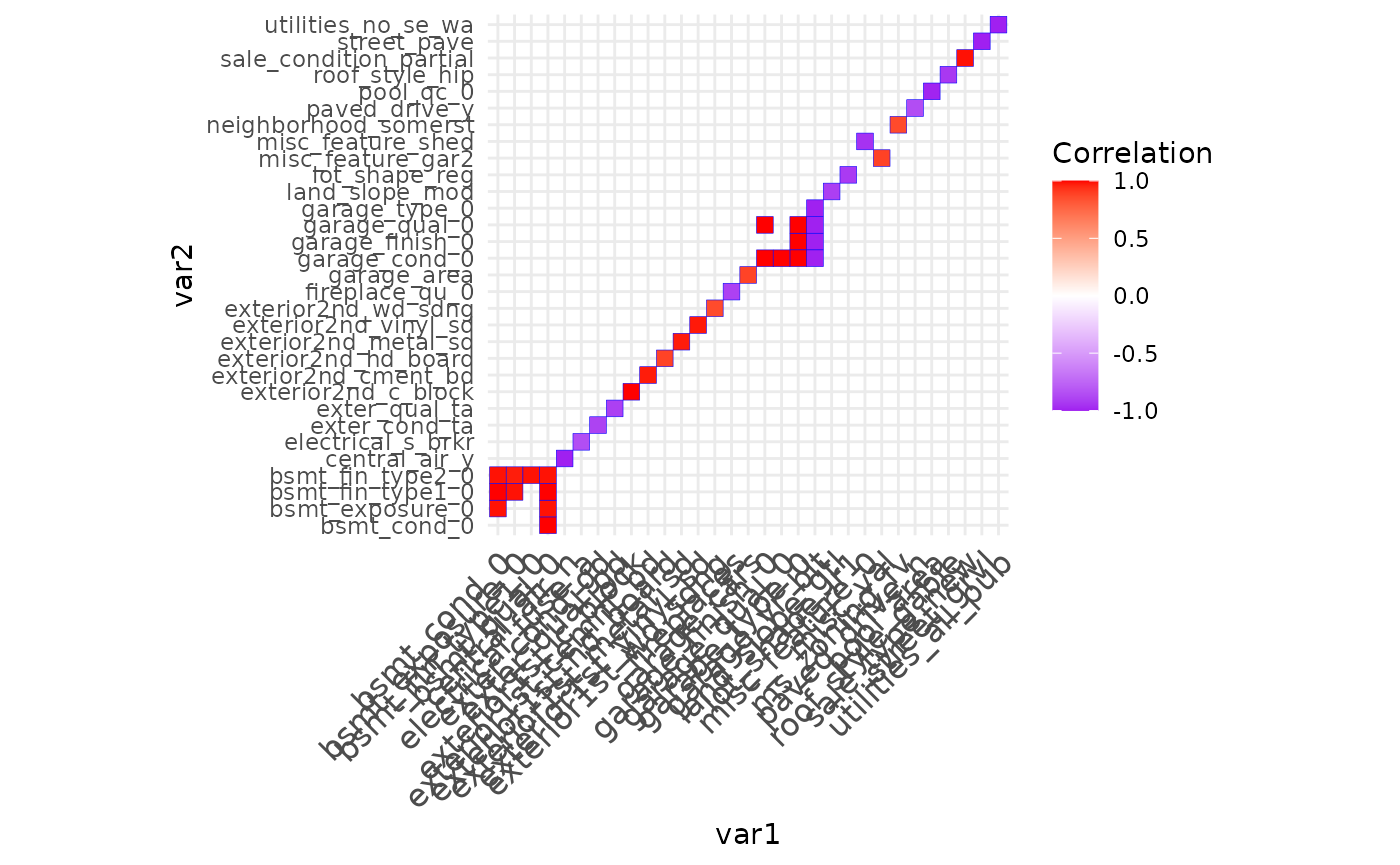
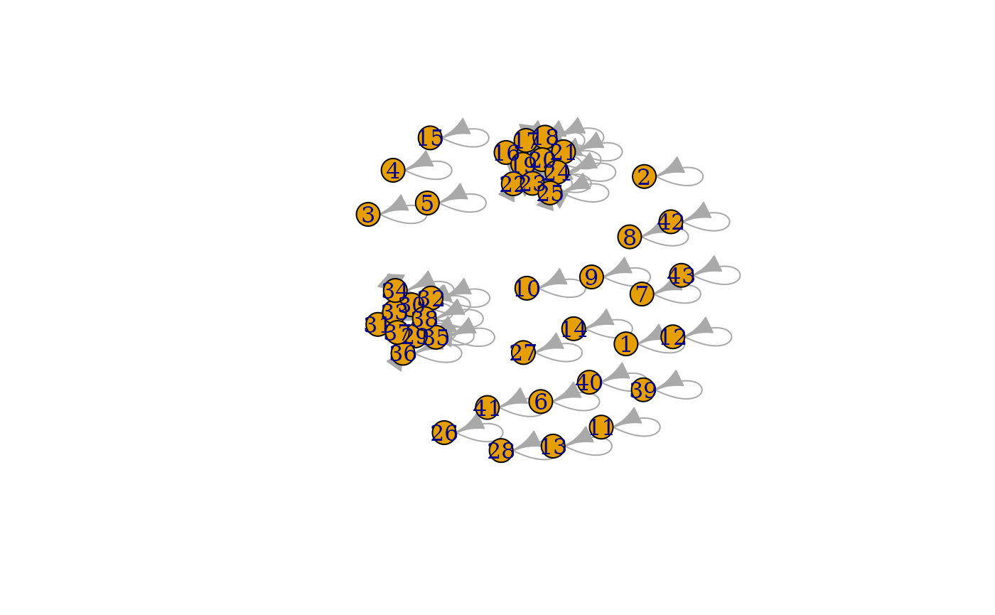
For visualization purposes, we are only working with the top 20 variables. We can take the various relationships and visualize them on a single graph. TangledFeatures also returns the variables as well as the correlation metric used between them.
From the graph we can broadly see that there are two clusters of interrelated variables, basement related variables and garage related variables. Additionally there are smaller clusters.
Igraph_plot <- Results$Graph_plot
plot(Igraph_plot)
TangledFeatures uses graph theory algorithms to define clusters of interrelated variables. From the network plot we can see the two clusters that we observed in the heatmap, as well as a few other clusters.
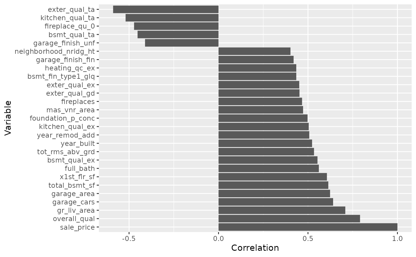
Let’s see the correlation between the sales price and the other variables. We are plotting only significant correlations above 0.4 and below -0.4 for space.
cor_df <- as.data.frame(sort(cor(Data$Cleaned_Data)[,37]))
cor_df$Correlation <- cor_df[,1]
cor_df <- cor_df[c(-1)]
cor_df$Variable <- rownames(cor_df)
rownames(cor_df) <- NULL


cor_df_subset <- cor_df[abs(cor_df$Correlation) > 0.4,]
cor_df_subset <- cor_df_subset[order(-cor_df_subset$Correlation), ]
rownames(cor_df_subset) <- NULL
cor_df_subset$Variable <- as.factor(cor_df_subset$Variable)

p <- ggplot(data = cor_df_subset, aes(x = Correlation, y = Variable)) +
            geom_bar(stat="identity") +
            scale_y_discrete(limits = cor_df_subset$Variable)

plot(p)
Although simple correlation is of course not indicative of a variable’s behavior in a linear model, this is a good starting place to see the relationships. Both garage and basement variables have both positive and negative relationships on the dependent variable. Let’s observe the positive relationship of Garage Area and the Sale price.
Features selected by TangledFeatures
TangledFeatures_variables <- Results$Final_VariablesLet us input the given features into a linear model and observe the behavior
formula_TangledFeatures <- as.formula(paste(paste("sale_price", '~'), paste(TangledFeatures_variables, collapse = "+")))
lm_TangledFeatures <- lm(formula_TangledFeatures, data = Data$Cleaned_Data)

summary(lm_TangledFeatures)
#>
#> Call:
#> lm(formula = formula_TangledFeatures, data = Data$Cleaned_Data)
#>
#> Residuals:
#>     Min      1Q  Median      3Q     Max
#> -509617  -16390    -986   13888  266668
#>
#> Coefficients:
#>                  Estimate Std. Error t value Pr(>|t|)
#> (Intercept)    -1.056e+06  1.147e+05  -9.206  < 2e-16 ***
#> overall_qual    1.674e+04  1.147e+03  14.595  < 2e-16 ***
#> gr_liv_area     5.093e+01  2.430e+00  20.960  < 2e-16 ***
#> year_built      2.438e+02  4.501e+01   5.417 7.10e-08 ***
#> total_bsmt_sf   2.282e+01  2.764e+00   8.258 3.30e-16 ***
#> garage_area     3.959e+01  5.874e+00   6.738 2.30e-11 ***
#> year_remod_add  2.672e+02  6.061e+01   4.408 1.12e-05 ***
#> bsmt_qual_ex    4.948e+04  4.014e+03  12.326  < 2e-16 ***
#> ---
#> Signif. codes:  0 '***' 0.001 '**' 0.01 '*' 0.05 '.' 0.1 ' ' 1
#>
#> Residual standard error: 36350 on 1452 degrees of freedom
#> Multiple R-squared:  0.7917, Adjusted R-squared:  0.7906
#> F-statistic: 788.2 on 7 and 1452 DF,  p-value: < 2.2e-16
The features selected all seem to indicate significance and more importantly agree with the findings from our correlation analysis.
Let’s see what simple Lasso gives
library(caret)
library(glmnet)

control = caret::trainControl(method = "cv",number=5)

set.seed(849)
lasso_caret <- caret::train(x = Data$Cleaned_Data[ , -c("sale_price")], y = Data$Cleaned_Data$sale_price, method = "glmnet",
                trControl=control, preProc = c("center","scale"),
                tuneGrid = expand.grid(alpha = 1,
                                       lambda = 0))

lasso_coef <- coef(lasso_caret$finalModel,lasso_caret$bestTune$lambda)
Let’s run a linear model with the variables we get from lasso
lasso_coef <- as.data.frame(as.matrix(lasso_coef))
lasso_coef$Var_names <- rownames(lasso_coef)

lasso_variables <- lasso_coef[which(lasso_coef$s1 > 0),]$Var_names

formula_lasso <- as.formula(paste(paste("sale_price", '~'), paste(lasso_variables[-1], collapse = "+")))
lm_lasso <- lm(formula_lasso, data = Data$Cleaned_Data)

summary(lm_lasso)
#>
#> Call:
#> lm(formula = formula_lasso, data = Data$Cleaned_Data)
#>
#> Residuals:
#>     Min      1Q  Median      3Q     Max
#> -310125  -11206     300   10830  243571
#>
#> Coefficients: (1 not defined because of singularities)
#>                           Estimate Std. Error t value Pr(>|t|)
#> (Intercept)             -1.494e+06  1.854e+05  -8.061 1.68e-15 ***
#> lot_frontage            -1.631e+01  2.468e+01  -0.661 0.508981
#> lot_area                 3.728e-01  9.113e-02   4.090 4.57e-05 ***
#> overall_qual             7.642e+03  1.067e+03   7.160 1.34e-12 ***
#> overall_cond             5.346e+03  9.229e+02   5.792 8.68e-09 ***
#> year_built               2.957e+02  6.762e+01   4.374 1.32e-05 ***
#> year_remod_add           6.050e+01  5.848e+01   1.034 0.301109
#> mas_vnr_area             1.157e+01  5.239e+00   2.209 0.027330 *
#> bsmt_fin_sf1             6.080e+00  2.863e+00   2.124 0.033895 *
#> bsmt_fin_sf2             5.939e+00  8.850e+00   0.671 0.502286
#> total_bsmt_sf            5.306e+00  4.858e+00   1.092 0.274891
#> x2nd_flr_sf              1.294e+01  6.577e+00   1.968 0.049270 *
#> gr_liv_area              4.193e+01  5.747e+00   7.295 5.12e-13 ***
#> bsmt_full_bath           6.152e+03  2.073e+03   2.968 0.003048 **
#> full_bath                6.784e+03  2.315e+03   2.931 0.003442 **
#> half_bath                1.951e+03  2.283e+03   0.854 0.393111
#> tot_rms_abv_grd          2.013e+03  8.992e+02   2.239 0.025315 *
#> fireplaces               6.717e+03  2.919e+03   2.301 0.021544 *
#> garage_cars              8.637e+03  2.400e+03   3.599 0.000331 ***
#> garage_area             -2.135e+00  8.145e+00  -0.262 0.793295
#> wood_deck_sf             1.215e+01  6.653e+00   1.826 0.068061 .
#> open_porch_sf           -1.893e+01  1.277e+01  -1.483 0.138354
#> enclosed_porch           1.751e+01  1.393e+01   1.256 0.209261
#> x3ssn_porch              3.536e+01  2.508e+01   1.410 0.158799
#> screen_porch             5.370e+01  1.389e+01   3.866 0.000116 ***
#> pool_area                1.121e+03  1.449e+02   7.738 1.98e-14 ***
#> misc_val                -8.996e-02  1.607e+00  -0.056 0.955353
#> ms_zoning_fv             6.025e+03  7.526e+03   0.801 0.423541
#> alley_grvl               3.559e+02  4.508e+03   0.079 0.937075
#> lot_shape_ir2            7.225e+03  4.714e+03   1.533 0.125578
#> lot_shape_ir3           -2.439e+04  9.427e+03  -2.588 0.009768 **
#> land_contour_hls         5.743e+03  4.395e+03   1.307 0.191599
#> utilities_all_pub        1.910e+04  2.873e+04   0.665 0.506327
#> lot_config_corner        2.021e+03  1.973e+03   1.025 0.305765
#> lot_config_cul_d_sac     1.021e+04  3.348e+03   3.048 0.002349 **
#> land_slope_mod           3.222e+03  3.981e+03   0.809 0.418491
#> neighborhood_blmngtn     1.065e+04  7.619e+03   1.398 0.162308
#> neighborhood_blueste     7.605e+03  2.009e+04   0.379 0.705017
#> neighborhood_br_dale     1.472e+04  8.032e+03   1.832 0.067114 .
#> neighborhood_brk_side    1.308e+04  4.379e+03   2.987 0.002868 **
#> neighborhood_crawfor     2.716e+04  4.527e+03   5.999 2.56e-09 ***
#> neighborhood_meadow_v    7.828e+03  8.985e+03   0.871 0.383788
#> neighborhood_no_ridge    5.151e+04  5.217e+03   9.872  < 2e-16 ***
#> neighborhood_n_pk_vill   2.403e+04  9.833e+03   2.444 0.014671 *
#> neighborhood_nridg_ht    3.936e+04  4.425e+03   8.896  < 2e-16 ***
#> neighborhood_sawyer_w    9.515e+03  3.962e+03   2.401 0.016471 *
#> neighborhood_somerst     1.790e+04  6.810e+03   2.628 0.008677 **
#> neighborhood_stone_br    5.795e+04  6.221e+03   9.316  < 2e-16 ***
#> neighborhood_swisu      -6.636e+01  6.130e+03  -0.011 0.991365
#> neighborhood_veenker     1.401e+04  8.902e+03   1.574 0.115686
#> condition1_norm          1.110e+04  2.589e+03   4.287 1.94e-05 ***
#> condition1_pos_n        -1.063e+04  7.020e+03  -1.515 0.130124
#> condition1_rr_an         1.290e+04  6.436e+03   2.004 0.045295 *
#> condition2_artery       -6.298e+03  2.174e+04  -0.290 0.772117
#> condition2_feedr        -9.284e+03  1.254e+04  -0.740 0.459183
#> condition2_pos_a         7.244e+04  3.508e+04   2.065 0.039128 *
#> condition2_rr_nn        -6.379e+02  2.006e+04  -0.032 0.974637
#> bldg_type_1fam           2.620e+04  2.983e+03   8.782  < 2e-16 ***
#> bldg_type_2fm_con        1.161e+04  6.506e+03   1.785 0.074455 .
#> house_style_1_5unf       1.855e+04  8.792e+03   2.110 0.035031 *
#> house_style_1story       1.844e+04  3.883e+03   4.749 2.27e-06 ***
#> house_style_s_foyer      1.008e+04  6.153e+03   1.638 0.101660
#> house_style_s_lvl        4.487e+03  4.965e+03   0.904 0.366312
#> roof_style_gambrel      -4.292e+03  9.057e+03  -0.474 0.635663
#> roof_style_mansard       1.045e+04  1.124e+04   0.930 0.352487
#> roof_style_shed          1.789e+04  2.097e+04   0.853 0.393564
#> roof_matl_membran        3.339e+04  2.935e+04   1.137 0.255547
#> roof_matl_metal          1.283e+04  2.803e+04   0.458 0.647148
#> roof_matl_tar_grv       -2.425e+04  9.555e+03  -2.538 0.011278 *
#> roof_matl_wd_shngl       7.803e+04  1.216e+04   6.418 1.92e-10 ***
#> exterior1st_asb_shng     2.036e+03  6.893e+03   0.295 0.767752
#> exterior1st_brk_comm     1.183e+04  2.086e+04   0.567 0.570851
#> exterior1st_brk_face     2.141e+04  4.435e+03   4.826 1.55e-06 ***
#> exterior1st_cemnt_bd     6.461e+03  1.671e+04   0.387 0.699072
#> exterior1st_metal_sd     5.094e+03  2.662e+03   1.913 0.055908 .
#> exterior1st_stone        9.264e+03  2.091e+04   0.443 0.657803
#> exterior1st_stucco      -3.338e+03  6.428e+03  -0.519 0.603627
#> exterior1st_wd_shing    -5.589e+02  5.873e+03  -0.095 0.924191
#> exterior2nd_asph_shn     4.162e+03  1.666e+04   0.250 0.802795
#> exterior2nd_cment_bd    -1.679e+03  1.696e+04  -0.099 0.921181
#> exterior2nd_im_stucc     3.111e+04  9.098e+03   3.419 0.000647 ***
#> exterior2nd_vinyl_sd     6.990e+03  2.497e+03   2.799 0.005197 **
#> exterior2nd_wd_sdng      2.532e+03  2.714e+03   0.933 0.351090
#> mas_vnr_type_stone       6.489e+02  3.092e+03   0.210 0.833813
#> exter_qual_ex            1.068e+04  5.465e+03   1.954 0.050924 .
#> exter_qual_fa            6.099e+01  8.876e+03   0.007 0.994519
#> exter_cond_ex            6.273e+03  1.995e+04   0.314 0.753273
#> exter_cond_fa            2.618e+03  6.386e+03   0.410 0.681929
#> exter_cond_po            4.701e+03  2.875e+04   0.163 0.870156
#> foundation_p_conc        6.964e+02  2.504e+03   0.278 0.780928
#> foundation_stone         2.800e+03  1.191e+04   0.235 0.814199
#> bsmt_qual_0              1.866e+03  8.004e+03   0.233 0.815717
#> bsmt_qual_ex             2.386e+04  3.706e+03   6.438 1.69e-10 ***
#> bsmt_qual_fa             2.396e+03  5.270e+03   0.455 0.649434
#> bsmt_cond_po             1.600e+04  2.236e+04   0.715 0.474496
#> bsmt_exposure_av         6.565e+03  2.406e+03   2.729 0.006442 **
#> bsmt_exposure_gd         2.190e+04  3.304e+03   6.628 4.94e-11 ***
#> bsmt_fin_type1_0                NA         NA      NA       NA
#> bsmt_fin_type1_blq       4.818e+03  2.653e+03   1.816 0.069635 .
#> bsmt_fin_type1_glq       8.121e+03  2.396e+03   3.390 0.000720 ***
#> bsmt_fin_type2_alq       7.718e+03  7.350e+03   1.050 0.293891
#> bsmt_fin_type2_glq       3.270e+02  9.026e+03   0.036 0.971104
#> bsmt_fin_type2_unf       1.193e+03  4.010e+03   0.298 0.766021
#> heating_gas_a           -1.115e+03  6.082e+03  -0.183 0.854535
#> heating_wall             7.734e+03  1.601e+04   0.483 0.629109
#> heating_qc_ex            2.811e+03  1.940e+03   1.449 0.147545
#> heating_qc_fa           -1.120e+03  4.595e+03  -0.244 0.807536
#> heating_qc_po           -2.082e+04  2.923e+04  -0.712 0.476349
#> electrical_0             1.212e+04  2.758e+04   0.439 0.660473
#> electrical_fuse_f        3.391e+02  5.987e+03   0.057 0.954840
#> kitchen_qual_ex          2.694e+04  3.930e+03   6.854 1.10e-11 ***
#> kitchen_qual_fa          1.470e+03  5.378e+03   0.273 0.784665
#> functional_min2          6.305e+03  6.093e+03   1.035 0.300948
#> functional_typ           1.477e+04  3.996e+03   3.695 0.000229 ***
#> fireplace_qu_0           2.840e+03  3.724e+03   0.763 0.445763
#> fireplace_qu_po          5.660e+03  6.515e+03   0.869 0.385159
#> garage_type_basment     -3.744e+03  6.973e+03  -0.537 0.591425
#> garage_type_car_port     3.354e+03  1.004e+04   0.334 0.738266
#> garage_type_detchd       5.848e+02  2.277e+03   0.257 0.797350
#> garage_finish_fin        1.330e+03  2.050e+03   0.648 0.516794
#> garage_qual_ex           2.552e+04  1.688e+04   1.511 0.130951
#> garage_cond_po          -1.678e+04  1.172e+04  -1.432 0.152520
#> paved_drive_n           -8.943e+02  3.652e+03  -0.245 0.806564
#> pool_qc_0                6.574e+05  8.534e+04   7.703 2.59e-14 ***
#> fence_mn_prv             3.470e+03  2.496e+03   1.390 0.164775
#> misc_feature_othr        7.702e+03  2.040e+04   0.378 0.705783
#> misc_feature_shed       -1.074e+03  4.397e+03  -0.244 0.807092
#> sale_type_con            2.957e+04  1.992e+04   1.484 0.137968
#> sale_type_con_ld         1.005e+04  9.752e+03   1.031 0.302836
#> sale_type_con_li         6.460e+03  1.239e+04   0.521 0.602232
#> sale_type_cwd            1.622e+04  1.416e+04   1.145 0.252409
#> sale_type_new            1.833e+04  4.139e+03   4.429 1.03e-05 ***
#> sale_type_oth            9.270e+03  1.627e+04   0.570 0.569019
#> sale_condition_adj_land  2.705e+04  1.480e+04   1.827 0.067932 .
#> sale_condition_alloca   -7.798e+03  9.184e+03  -0.849 0.395961
#> sale_condition_normal    6.808e+03  2.766e+03   2.461 0.013970 *
#> ---
#> Signif. codes:  0 '***' 0.001 '**' 0.01 '*' 0.05 '.' 0.1 ' ' 1
#>
#> Residual standard error: 26970 on 1325 degrees of freedom
#> Multiple R-squared:  0.8953, Adjusted R-squared:  0.8848
#> F-statistic: 84.59 on 134 and 1325 DF,  p-value: < 2.2e-16
There are clearly a lot of variables. Most of them are insignificant and the coefficient direction varies wildly from what we have seen in correlation. This is a fairly bad model that seems to be significantly over fitting.
Let’s see what Random Forest RFE gives
control <- caret::rfeControl(functions = rfFuncs,
                      method = "repeatedcv", # repeated cv
                      repeats = 2, # number of repeats
                      number = 2) # number of folds


result_rfe <- caret::rfe(x = Data$Cleaned_Data[ , -c("sale_price")],
                   y = Data$Cleaned_Data$sale_price,
                   sizes = c(1:35),
                   rfeControl = control)
result_rfe <- predictors(result_rfe)
This is about 10x slower than TangledFeatures. Let’s see the variable behavior in a linear model.
formula_rfe <- as.formula(paste(paste("sale_price", '~'), paste(result_rfe, collapse = "+")))
lm_rfe <- lm(formula_rfe, data = Data$Cleaned_Data)

summary(lm_rfe)
#>
#> Call:
#> lm(formula = formula_rfe, data = Data$Cleaned_Data)
#>
#> Residuals:
#>     Min      1Q  Median      3Q     Max
#> -484453  -15025   -1020   13777  274307
#>
#> Coefficients:
#>                        Estimate Std. Error t value Pr(>|t|)
#> (Intercept)          -1.202e+06  1.551e+05  -7.751 1.73e-14 ***
#> gr_liv_area           1.846e+01  1.901e+01   0.971 0.331743
#> overall_qual          1.682e+04  1.153e+03  14.592  < 2e-16 ***
#> total_bsmt_sf         1.056e+01  6.719e+00   1.572 0.116159
#> bsmt_fin_sf1          6.962e+00  5.818e+00   1.197 0.231626
#> x2nd_flr_sf           3.007e+01  1.922e+01   1.564 0.117972
#> x1st_flr_sf           2.529e+01  1.947e+01   1.299 0.194262
#> garage_cars           1.719e+04  2.905e+03   5.917 4.10e-09 ***
#> garage_area          -2.292e+00  9.563e+00  -0.240 0.810609
#> year_built            4.050e+02  6.614e+01   6.123 1.18e-09 ***
#> lot_area              4.318e-01  9.823e-02   4.395 1.19e-05 ***
#> exter_qual_ta        -4.192e+04  5.165e+03  -8.116 1.03e-15 ***
#> year_remod_add        2.002e+02  6.622e+01   3.023 0.002544 **
#> overall_cond          5.358e+03  1.018e+03   5.264 1.63e-07 ***
#> tot_rms_abv_grd      -6.810e+02  1.037e+03  -0.657 0.511415
#> garage_yr_blt        -1.025e+01  3.264e+00  -3.140 0.001723 **
#> ms_zoning_rm         -3.608e+03  4.554e+03  -0.792 0.428427
#> ms_sub_class         -1.627e+02  2.484e+01  -6.551 7.94e-11 ***
#> neighborhood_crawfor  2.505e+04  5.167e+03   4.847 1.39e-06 ***
#> fireplace_qu_0       -5.575e+02  4.335e+03  -0.129 0.897692
#> garage_type_detchd    1.502e+03  4.162e+03   0.361 0.718320
#> full_bath             3.244e+03  2.728e+03   1.189 0.234573
#> kitchen_qual_gd      -7.413e+03  2.502e+03  -2.963 0.003100 **
#> garage_type_attchd   -1.188e+03  3.491e+03  -0.340 0.733766
#> bsmt_unf_sf          -2.830e+00  5.908e+00  -0.479 0.631963
#> mas_vnr_area          2.027e+01  5.854e+00   3.463 0.000550 ***
#> open_porch_sf        -1.349e+00  1.476e+01  -0.091 0.927189
#> ms_zoning_rl          1.136e+03  4.041e+03   0.281 0.778738
#> half_bath            -1.003e+03  2.584e+03  -0.388 0.697897
#> wood_deck_sf          2.910e+01  7.625e+00   3.816 0.000142 ***
#> garage_finish_unf    -2.190e+03  2.632e+03  -0.832 0.405543
#> fireplaces            5.210e+03  3.419e+03   1.524 0.127851
#> exter_qual_gd        -2.808e+04  5.092e+03  -5.515 4.13e-08 ***
#> bsmt_full_bath        9.431e+03  2.407e+03   3.917 9.38e-05 ***
#> bsmt_qual_gd         -1.212e+04  2.447e+03  -4.954 8.12e-07 ***
#> central_air_n         1.597e+03  4.274e+03   0.374 0.708755
#> ---
#> Signif. codes:  0 '***' 0.001 '**' 0.01 '*' 0.05 '.' 0.1 ' ' 1
#>
#> Residual standard error: 33390 on 1424 degrees of freedom
#> Multiple R-squared:  0.8276, Adjusted R-squared:  0.8233
#> F-statistic: 195.2 on 35 and 1424 DF,  p-value: < 2.2e-16
Although a little better than lasso, we still have many variables that are insignificant. Variables such as garage_area having a negative coefficient also do not make sense.
Comparisons
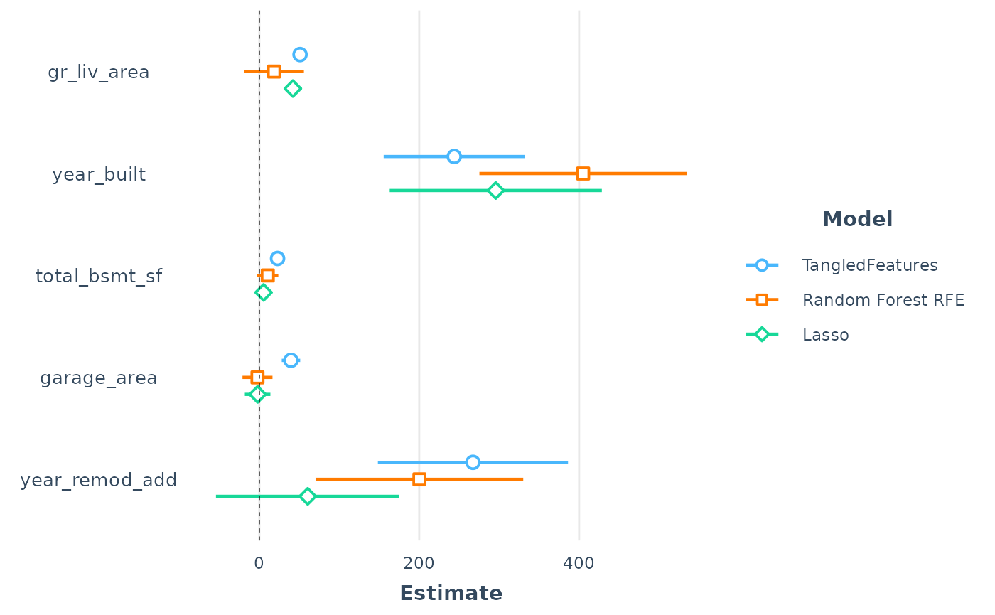
If we take a look at the coefficient behavior across three models for a few variables, we can see that it is largely the same with one major exception.
jtools::plot_summs(lm_TangledFeatures, lm_rfe, lm_lasso , coefs =
                   names(lm_TangledFeatures$coef)[! names(lm_TangledFeatures$coef) %in% c(("(Intercept)"),                        "overall_qual", "bsmt_qual_ex")],
                   model.names = c("TangledFeatures", "Random Forest RFE", "Lasso"))
We can see the coefficients as well as the confidence intervals for each linear model.
Both Lasso and Random Forest make the garage_area variable negative, as it is highly correlated with other variables. TangledFeatures takes the variable interrelationships into account and generates the correct variable effect. The confidence interval for the model from TangledFeatures is tighter as well.
Conclusion
We have seem the effects variables from TangledFeatures has on the outcome compared to a few other simple feature techniques. There are many ways to pick features for a linear/logistic model. As of right now, TangledFeatures is the best alternative to traditional dimensionality reduction techniques.